Feedforward network (FFN) blocks are the least talked about elements in the context of LLMs, but they are where more than 70% of the parameters originate. Something as simple and convenient as a couple of linear transformation matrices becomes a burden when models start scaling into billions of parameters. Thus, getting the maximum juice out of a lean structure is a challenge. FFNs are mostly under-represented in discussions even if the sub-layer acts as the primary “knowledge” processing engine, processing all the meaningful contexts activation layer has provided it.
🔥 Standard Position-Wise Feedforward Network
This is as simple as it gets: a two-layered fully connected network of neurons with a single activation switch—most probably a ReLU variant (for LLMs).
$$ FFN(x) = \max(0, xW_1 + b_1)W_2 + b_2 $$
The same transformation is applied to each token in parallel, making it efficient for GPU computation. For example, in the BERT model, the 512 dimensions of each token are expanded to 2048 to allow for “intricate interactions” before projecting back to 512 dimensions. This expansion/contraction is crucial; in every transformer, stacking of layers is possible only because the output of every layer matches its input dimensions.
🔥 SWiGLU
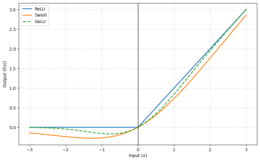
Sigmoid Weighted Gated Linear Unit (SWiGLU) has become the gold standard for feedforward networks in LLMs like Llama 3 and PaLM. The primary reasons for choosing the Swish function (shown in the first image) over ReLU or GELU are as follows:
- Mathematical Linearity: Swish (SiLU) is defined as $x \cdot \text{sigmoid}(\beta x)$, where $\beta$ is a learnable parameter. It is a smooth, non-monotonic function that allows small negative values to pass through. While GELU ($x \cdot \Phi(x)$) is also smooth, Swish’s specific curve has empirically improved model performance.
- Computational Efficiency: SiLU gradients are simpler to compute ($x / (1 + \exp(-x))$) compared to standard GELU approximations. At the massive scale of modern LLMs, these shortcuts save significant training time.
- Performance: Research in the PaLM and Llama papers found that Swish-based Gated Linear Units consistently outperformed GELU-based versions in terms of perplexity and downstream task accuracy.
$$SwiGLU(x, W, V, b, c) = (\text{Swish}(xW + b) \otimes (xV + c))W_2$$
Where $W$ and $V$ are weight matrices for the gate and the data path, and $\otimes$ is element-wise multiplication.
- More Complex Filtering: Instead of using two weight matrices as in a standard FFN, SWiGLU uses three (gate, data, and output). This allows it to extract more complex features without a drastic increase in parameters. Modern implementations often lower the dimensionality of hidden layers (to ~2/3 of what they would be in a standard FFN) while retaining the performance benefits.
- Zero-Gradient Avoidance: Unlike ReLU, which has a zero gradient for all negative values (the “dying ReLU” problem), SwiGLU’s smooth curve ensures the model can still learn from negative inputs, improving training stability in deep stacks.
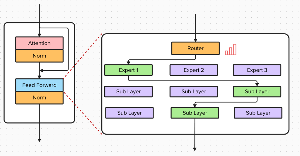
🔥 Mixture of Experts (MoE)
MoE is an entire architecture rather than just a single block. It has become the dominant strategy for scaling models to insane sizes—up to a trillion parameters (like DeepSeek-V3 and GPT-4)—because it breaks the direct link between model size (information capacity) and speed (inference cost).
- Sparse Activation: MoE uses a “Router” to determine which smaller “Experts” (specialized FFNs) are best suited for a specific token. Instead of activating the entire network, only a tiny fraction of experts are used per token. For instance, DeepSeek-V3 might have 256 expert layers but only activate 8 for any single token.
- Big Scale, Small Compute: MoE allows “trillion-parameter intelligence” to run at the speed of a much smaller model. While DeepSeek-V3 has 671 billion total parameters, it only uses ~37 billion per token during inference. You get the reasoning performance of a massive model with the latency of a smaller one.
- Expert Specialization: Because different experts handle different tokens, they naturally specialize. Analysis shows certain experts become “specialists” in mathematics or coding, while others handle general language.
- Training Efficiency: Since you only update a fraction of the weights for each token, MoE models can process many more tokens per second during training compared to a dense model of the same total size.
Training Dynamics and instability: The router assigns probabilities to each expert. To avoid overfitting or “expert collapse” (where the router sends everything to one expert), noise is often added to the router’s output during training. Some models choose one top expert, while others choose multiple and average their outputs. This is called the “auxilliary loss free” strategy to controll training biases.
The Challenges of MoE
- The RAM Wall: Even if only a small percentage of parameters are used for computation, all 671B parameters must still reside in GPU memory. This makes MoE models difficult to run on consumer hardware.
- Communication Overhead: In distributed training, experts are often split across different GPUs. If a token on GPU 1 needs an expert on GPU 4, data must travel over the network. DeepSeek-V3 employs “Node-Limited Routing” to minimize this congestion.
Summary: MoE is the better choice for major labs (like DeepSeek, Google, or OpenAI) trying to maximize intelligence per dollar of training cost. Dense SwiGLU remains the standard for reliability, ease of deployment, and local execution.