According to the laws of hardware physics, training a Large Language Model (LLM) should be practically impossible. Still, we see these behemoths adopting new names and functions every day. The landscape of LLMs is defined by a singular overarching principle: the exponential scaling of model parameters and training datasets. The transition from models with hundreds of millions of parameters to those boasting trillions—such as GPT-4, Llama 3, and DeepSeek-V3—has fundamentally altered machine learning, from algorithmic design to massive-scale systems engineering. Training an LLM now requires an orchestration of thousands of accelerators, functioning as a unified supercomputer.
The Anatomy of a Parameter:
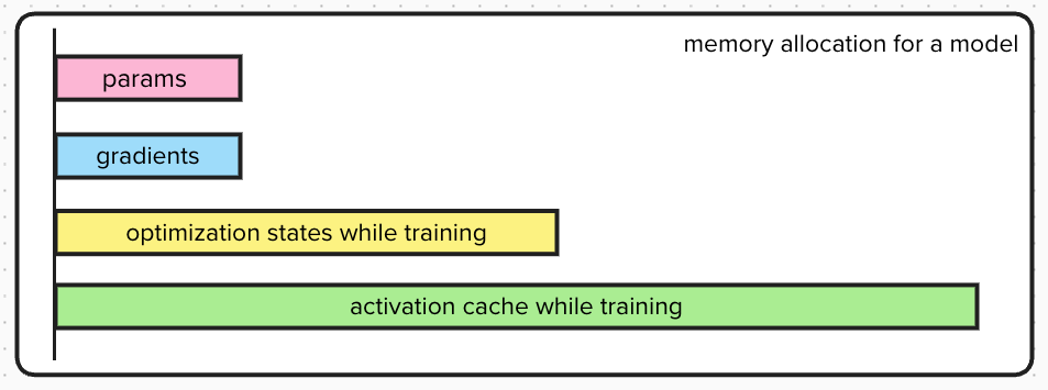
The memory consumption of an LLM is not a storage tool for model weights only. It is a standard mixed-precision training environment that is dominated by these components:
Model Parameters (Weights): The raw matrices that define the model’s intelligence. In 16-bit precision (2 bytes per parameter), a 1-trillion parameter model requires 2 Terabytes (TB) of storage just to load. For a 1T parameter model with FP16 precision, this is terabytes $2 \times 10^{12} = 2 T$ parameters.
Gradient Accumulation: During the backward pass, the gradient of the loss function with respect to every parameter must be calculated and stored. This mirrors the size of the parameters, adding another 2 TB for a 1T model. For a 1T parameter model will have 1T gradients with FP16 precision, this is terabytes $2 \times 10^{12} = 2 T$.
Optimizer States: This is often the largest consumer of memory. Modern optimizers like Adam require maintaining the momentum (first moment) and variance (second moment) for every parameter to guide the gradient descent. These are typically stored in high precision (FP32). For a model with $\Psi$ parameters, Adam requires 12 bytes per parameter (4 bytes for the master weight copy, 4 bytes for momentum, 4 bytes for variance). For a 1T model, this is 12 TB. The reason for storing high precision values is to help the gradient change even for the very small increments in the parameters. For a 1T model, this is terabytes $12 \times 10^{12} = 12 T$.
Activation Cache: Activations are the intermediate outputs stashed during the forward pass to be used later in the backward pass (backpropagation). Unlike static memory, this scales with Batch Size and Sequence Length (Context Window).
The Scaling Law: Activation memory is often defined by:$$\text{Memory}_{act} = \text{Batch Size} \times \text{Sequence Length} \times \text{Hidden Dimension} \times \text{Num Layers}$$
For Compute: 2 FLOPS for Forward Pass (for tokens), 4 FLOPs for backward pass (for tokens and weights), with model size of 1T parameters and training dataset of 10T tokens,
$$FLOPs = 6 \times 10T \times 1T$$
A single H100 GPU offers 4000 TFLOPS per second as a theoretical maximum capacity. With this, it would take a single GPU over 400 years to train a 1T parameter model. That is why clusters of thousands of GPUs (10,000+) are used to train LLMs in a few months.
Data Parallelism (DDP): The “Naive” Approach
To understand this concept, let’s consider a simple example: the exam grading analogy. A professor (central model) is tasked with grading 1,000 students’ exams. He has 10 assistants (workers) to help him. He divides the exams into 10 batches of 100 exams each. He assigns each assistant to grade one batch of exams independently.
The process is as follows: 1. Replication: Each assistant has an identical copy of the answer key (model parameters). 2. Scatter (Partitioning): Each assistant gets a batch of exams to grade. 3. Compute: Each assistant grades their batch of exams independently. They mark errors, calculate scores, and make necessary score adjustments (gradients). During this process, there is no communication between the assistants. 4. Synchronization: A critical bottleneck. If assistant 1 and assistant 2 decide on different answers, there needs to be an aggregation process. At the end, all 10 assistants need to submit their answers to the professor, forming a long waiting queue before the next grading session begins.
In technical terms, this is called Data Parallelism. The model $M$ is replicated across $P$ devices. Each device $i$ processes a mini-batch of data $x_i \in D$, performs a forward pass to compute loss $L$, and a backward pass to compute gradients $g_i = \nabla L(x_i)$. The global gradient $G$ used to update the model is the average of all local gradients: $G = \frac{1}{P} \sum_{i=1}^{P} g_i$.
This replicates the traditional “Parameter Server” architecture. The next algorithm reduces the communication bottleneck by using “Ring All-Reduce”.
Synchronization Algorithm: Ring All-Reduce
This is a more P2P version of updating weights during training. Assume assistants are seated around the round table passing their batches to the next one all at once. Synchronization happens in two phases:
Scatter-Reduce: The gradients (the updates) are chopped into chunks. Assistant 1 passes the first chunk of numbers to Assistant 2, and Assistant 2 does the same with others. This travels a full circle and contains the sum of everyone’s updates. Multiple chunks circulate simultaneously like a conveyor belt.
All-Gather: Once the sums are computed they need to be broadcast to all the other assistants. The total sums continue to circulate the ring until every TA has a copy of the complete, aggregated gradient vector.
Mathematical Bandwidth Analysis:
The Ring All-Reduce optimizes the communication by reducing the number of communication rounds (bandwidth optimality). Let $N$ be the number of model parameters (and gradient vectors). Let $P$ be the number of GPUs.
In a naive central server architecture, the communication bandwidth scales with $P$. In the ring topology, the data is split into $P$ chunks of size $\frac{N}{P}$.
- Scatter-Reduce: Each GPU sends chunks of size $\frac{N}{P}$ to the next GPU exactly $P-1$ times. $$\text{Data Transferred per GPU} = (P-1) \times \frac{N}{P}$$
- All-Gather: Each GPU now aggregates with the received chunks for its $\frac{N}{P}$ from all other GPUs and aggregates it. Now these aggregated weights are broadcast to $P-1$ neighbors. $$\text{Data Transferred per GPU} = (P-1) \times \frac{N}{P}$$ Total Volume per communication round: $$V_{total} = 2 \times \frac{N(P-1)}{P}$$ As the number of GPUs $P$ tends to infinity, the Volume approaches $2N$. This is constant complexity. This property allows Data Parallelism to scale efficiently to massive clusters, limited only by the latency of the ring.
Breaking the Memory Wall: ZeRO and FSDP
Standard DDP requires each GPU to store the entire model’s parameters, gradients, and optimizer states. Standard H100 GPUs have 80 GB of HBM memory. This limitation led to the development of the Zero Redundancy Optimizer (ZeRO) by Microsoft DeepSpeed, and its PyTorch implementation, Fully Sharded Data Parallelism (FSDP).
Sharding vs Replication: In standard DDP, the model is replicated across all GPUs. In ZeRO, the model is sharded across GPUs. This means that while in DDP an encyclopedia is copied for all assistants, in ZeRO we tear it apart and distribute sections equally. Surprisingly, with respect to the compute-to-memory tradeoff, there is negligible loss. Collectively, the group possesses the full knowledge of the model, but no single individual carries the entire weight. When assistant 1 needs to grade a question requiring information from page 25, they request it from assistant 3. Assistant 3 broadcasts the page to everyone. Assistant 1 reads it, performs the calculation, and then immediately deletes it (freeing the memory). This allows the training of models far larger than individual GPU memory. ZeRO comes in three stages:
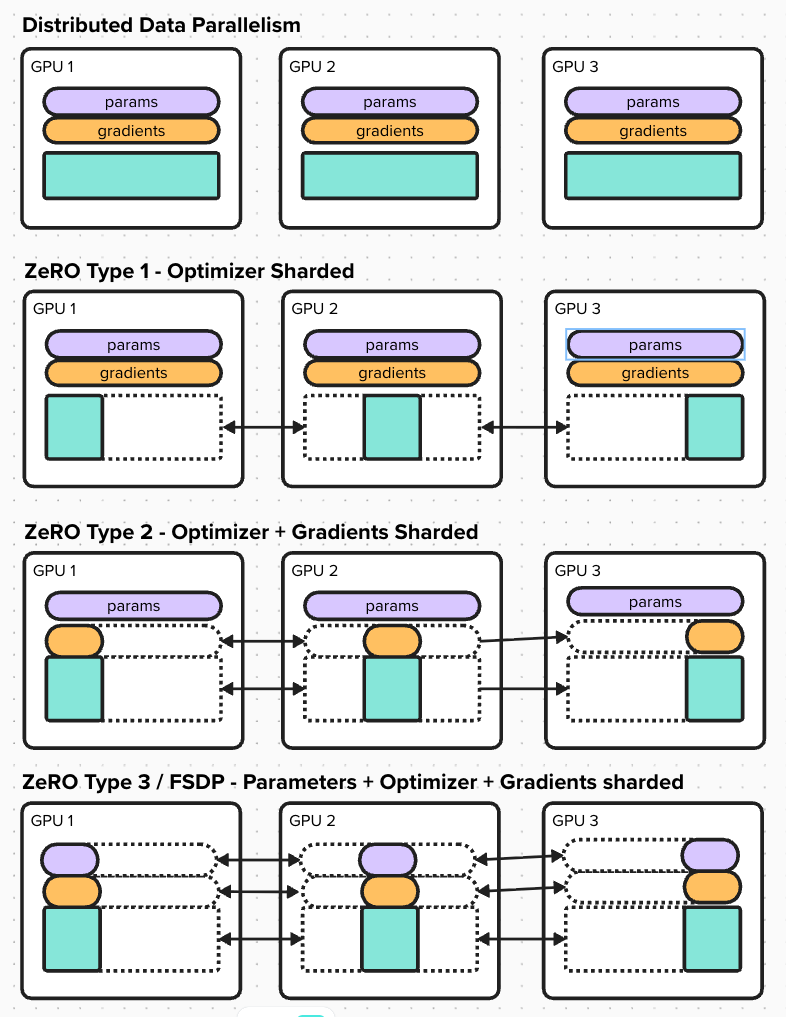
ZeRO Stage 1: In this stage, only the optimizer is sharded. The model parameters and gradients are replicated across all GPUs. During this process:
- A forward pass and backward pass are performed as in standard DDP. Then each model updates its section of weights from the sharded optimizer parameters locally. The update is then aggregated and broadcast to all GPUs. This is followed by all GPUs simultaneously.
ZeRO Stage 2: In this stage, the model gradients are also sharded. The model parameters are replicated across all GPUs. During this process:
- A forward pass is calculated independently on each GPU. While the backward passes are also calculated on the same GPU, the gradients belonging to the layers allotted to other GPUs are sent immediately to those GPUs and deleted immediately, freeing memory. The model only holds onto the gradients for its allotted layers and aggregates them with gradients received from other GPUs. The optimizer is then updated locally on each GPU, resulting in new weights for those layers.
- Once the new weights for partial layers are calculated, all GPUs broadcast their new weights to each other. This is followed by all GPUs simultaneously.
ZeRO Stage 3 (FSDP): This is the extreme case of model sharding, which increases compute time 1.5 times. In this stage, the model parameters are also sharded. During this process:
- In the forward pass, for each layer, the model parameters are brought from another GPU and loaded for the computation, then deleted immediately after. Each GPU only keeps parameters, gradients, and optimizer states for its partial layers.
In ZeRO-3, all these components are partitioned across $N_d$ devices. The memory consumption per device becomes:
For a 1-trillion parameter model ($\Psi = 10^{12}$), the total state memory is roughly 16 TB. DDP requires 16 TB per GPU (impossible). ZeRO-3 with 1024 GPUs: $\frac{16 \text{ TB}}{1024} \approx 16 \text{ GB}$. This 16 GB easily fits within the 80 GB limit of an A100/H100 GPU, leaving ample room for activation memory. This linear scaling capability is what enables the training of trillion-parameter models today.
This “gather-compute-discard” cycle could introduce massive latency. To mitigate this, FSDP employs prefetching. While the GPU is busy computing Layer $K$, the network interface (NIC) is simultaneously downloading the shards for Layer $K+1$. If the computation is heavy enough (which it is for large batch sizes), the communication time is effectively hidden, or “overlapped,” behind the computation. This relies heavily on high-bandwidth interconnects like NVIDIA’s NVLink or InfiniBand.
Here is a comparison of the memory requirements for ZeRO stages:
| ZeRO Stage | Optimization Target | Memory Reduction Factor | Communication Overhead |
|---|---|---|---|
| Stage 1 ($P_{os}$) | Optimizer States only | $4\times$ | Negligible (Same as DDP) |
| Stage 2 ($P_{os} + P_g$) | Optimizer + Gradients | $8\times$ | Negligible (Same as DDP) |
| Stage 3 ($P_{os} + P_g + P_p$) | Opt + Grad + Parameters | Linear with $N_d$ (Number of GPUs) | ~1.5x DDP |