Large language models arrive from pretraining with an extraordinary breadth of knowledge — language structure, facts, code, reasoning patterns — all learned from trillions of tokens of internet text. But this knowledge is unaligned. Ask a base model a question and you might get a continuation that reads like a Wikipedia paragraph, a Reddit comment, or a code snippet, with no coherent notion of “I should help this person.”
Supervised Fine-Tuning (SFT) is the stage that bridges that gap. By training on thousands of curated (instruction, response) pairs, we teach the model what good responses look like — turning a raw text-completion engine into something that follows instructions, holds conversations, and stays on task.
This post is a complete walkthrough of fine-tuning Llama 3.1 8B Instruct for a customer support domain using LoRA adapters on a single NVIDIA RTX 5090. We cover everything: dataset construction, the mechanics of loss masking, LoRA mathematics, training configuration, and a deep analysis of what 6,642 training steps actually did to the model’s internal representations.
The Full LLM Training Chain
Before diving in, it helps to understand where SFT sits in the broader training pipeline:
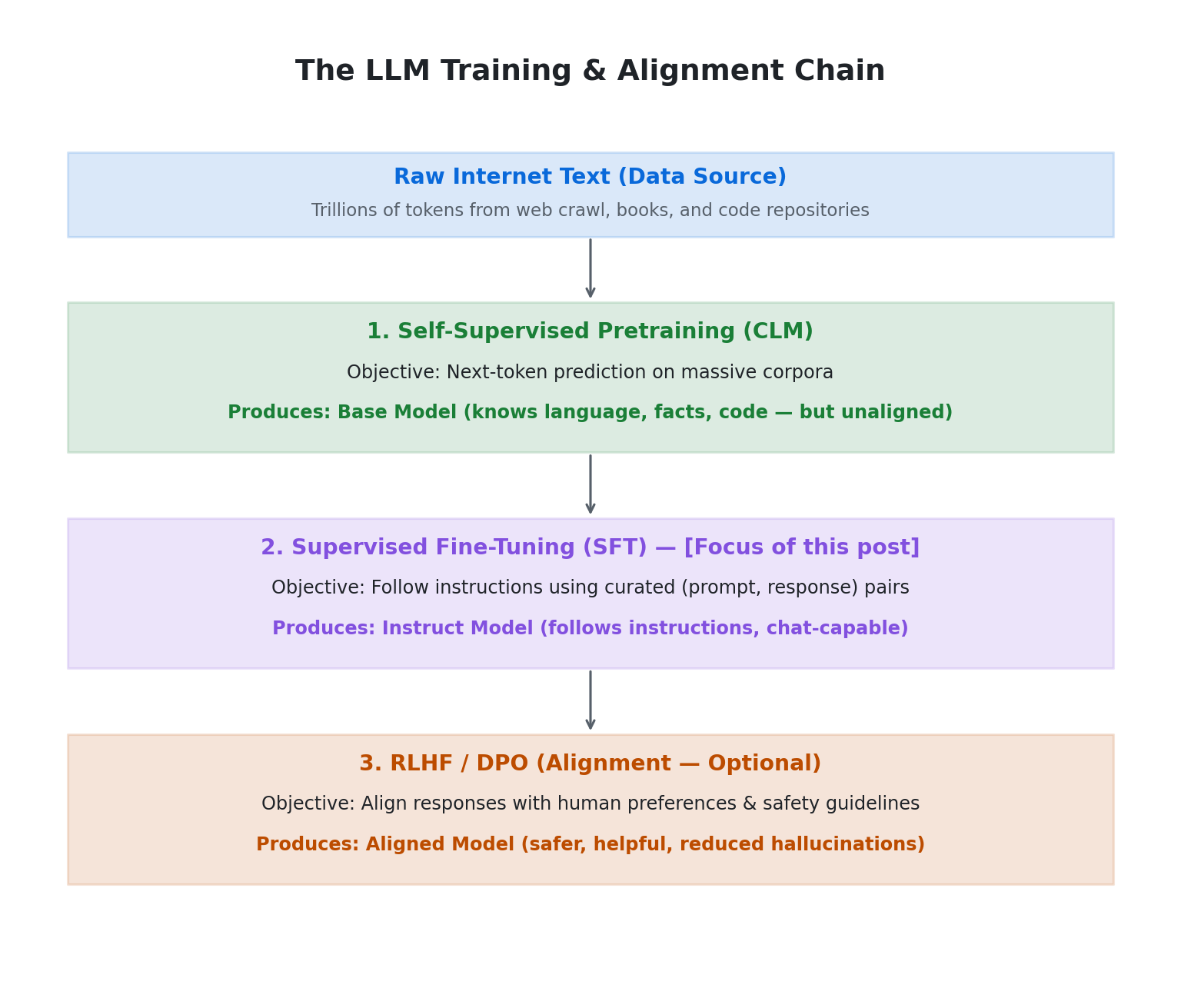
Both pretraining and SFT use Causal Language Modeling — the model predicts the next token given all previous tokens. The difference is in what they train on and where the loss is applied.
| Property | CLM (Pretraining) | SFT (Fine-Tuning) |
|---|---|---|
| Labels | Auto-generated from data itself | Human-curated (input, output) pairs |
| Supervision source | The data IS the label | External annotators or curated datasets |
| Data scale | Trillions of tokens | Thousands to millions of samples |
| Objective | Next token prediction | Produce desired output given input |
| Loss applied on | Every token in the sequence | Only the response/output tokens |
| Goal | Build world knowledge + language | Align behaviour to a task or instruction style |
| GPU cost | Enormous (weeks on thousands of GPUs) | Manageable (hours to days on a single GPU) |
Part 1: The Dataset
Source Data
We combine two complementary datasets for the customer support domain:
Bitext Customer Support LLM Chatbot Training Dataset — 53,744 single-turn instruction-response pairs spanning 27 intents across 11 categories:
| Category | Intents |
|---|---|
| Account | create_account, delete_account, edit_account, switch_account, recover_password |
| Order | cancel_order, change_order, place_order, track_order |
| Refund | track_refund, get_refund |
| Shipping | change_shipping_address, set_up_shipping_address, delivery_period |
| Payment | payment_issue, check_payment_methods |
| Subscription | newsletter_subscription |
| Contact | contact_customer_service, contact_human_agent |
| Feedback | complaint, review |
| Invoice | check_invoice, get_invoice |
| Cancellation | check_cancellation_fee |
| Registration | registration_problems |
MultiWOZ v2.2 — 8,437 multi-turn task-oriented dialogues across domains like restaurant booking, hotel search, taxi ordering, and train scheduling. Each dialogue contains multiple USER-SYSTEM turn pairs with rich slot-filling annotations.
The key insight: Bitext provides breadth (27 distinct customer intents with direct answers), while MultiWOZ adds what Bitext lacks — multi-turn context handling and slot-filling (extracting structured information like dates, prices, and locations from natural language).
Processing Pipeline
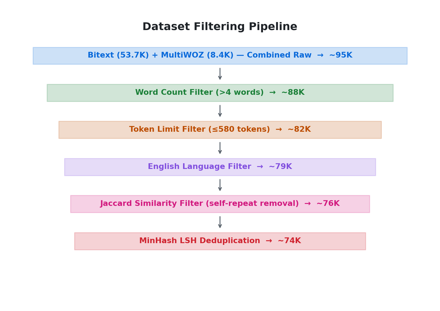
Raw data is noisy. Our filtering pipeline applies five sequential filters:
Step 1: Extract Instruction-Response Pairs
For MultiWOZ, we extract every consecutive USER→SYSTEM turn pair from each dialogue:
def multiwoz_to_instruction_response(dialogue_turns):
    """Convert MultiWOZ dialogue turns to instruction-response pairs."""
    pairs = []
    for i, turn in enumerate(dialogue_turns):
        if turn["speaker"] == "USER":
            if i + 1 < len(dialogue_turns) and dialogue_turns[i + 1]["speaker"] == "SYSTEM":
                pairs.append({
                    "instruction": turn["utterance"],
                    "response": dialogue_turns[i + 1]["utterance"]
                })
    return pairs
Bitext is already in (instruction, response) format, so it passes through directly.
Step 2: Word Count Filter
Trivially short samples (one or two-word queries like “Help” or “OK”) provide almost no learning signal and can actually hurt training by teaching the model that vague inputs deserve detailed responses:
def wc_filter_function(sample: dict) -> bool:
    query_wc = len(sample["instruction"].split())
    resp_wc = len(sample["response"].split())
    return query_wc > 4 and resp_wc > 5
Step 3: Token Limit Filter
We enforce a combined token limit of 580 tokens for the instruction + response pair. This is set below our training max_seq_length of 512 because the chat template adds system prompt tokens and special formatting tokens:
token_limit = 580
tokenizer = AutoTokenizer.from_pretrained("meta-llama/Llama-3.1-8b")

def tokenizer_filter_function(sample: dict) -> bool:
    tokens = tokenizer(
        sample["instruction"] + " " + sample["response"],
        truncation=False, add_special_tokens=True,
    )
    return len(tokens["input_ids"]) <= token_limit
Step 4: English Language Filter
MultiWOZ is English-only, but the Bitext dataset contains some multilingual noise. We use the lingua library for fast, accurate language detection:
from lingua import Language, LanguageDetectorBuilder

english_detect_algo = LanguageDetectorBuilder.from_languages(
    Language.ENGLISH, Language.CHINESE, Language.FRENCH,
).build()

def filter_english(sample: dict) -> bool:
    text = sample["instruction"] + sample["response"]
    lang = english_detect_algo.detect_language_of(text.replace("\n", ""))
    return lang == Language.ENGLISH
Step 5: Deduplication (Jaccard + MinHash LSH)
Customer support data is inherently repetitive — many variations of “How do I cancel my order?” map to nearly identical responses. We apply two deduplication stages:
First, a Jaccard similarity filter removes samples where the instruction and response are too similar to each other (a sign of parroting or template artifacts):
from nltk.metrics import jaccard_distance

def filter_same_inst_resp_pairs(sample: dict, threshold: float = 0.85) -> bool:
    instruction = set(sample["instruction"].lower().split())
    response = set(sample["response"].lower().split())
    similarity = 1 - jaccard_distance(instruction, response)
    return similarity < threshold
Then, MinHash LSH removes near-duplicate samples across the entire dataset:
from datasketch import MinHash, MinHashLSH

def dedup_dataset(dataset, threshold=0.8, num_perm=128, n_gram=5):
    lsh = MinHashLSH(threshold=threshold, num_perm=num_perm)
    keep_indices = []

    for idx, sample in enumerate(tqdm(dataset, desc="Deduplicating")):
        combined = sample["instruction"] + " " + sample["response"]
        m = get_minhash(combined, num_perm, n_gram)
        if not lsh.query(m):
            lsh.insert(str(idx), m)
            keep_indices.append(idx)

    return dataset.select(keep_indices)
Result: ~95K raw pairs → ~74K clean, deduplicated training samples (specifically 74,560 samples prior to the 95/5 train/validation split).
Part 2: Loss Masking — The Mechanism That Makes SFT Work
This is the single most important concept in SFT, and the one most commonly misunderstood.
The Problem
In SFT, each training sample is a single token sequence that looks like:
[system prompt tokens] [user message tokens] [assistant response tokens]
The model sees the entire sequence as input. During backpropagation, the default behavior is to compute loss on every token — meaning the model gets a training signal for predicting the system prompt and user message too.
Why that’s wrong: The system prompt and user message are things you wrote. You’re not trying to teach the model to reproduce them. You’re trying to teach it to produce the assistant response given the prompt. Training on prompt tokens wastes capacity and actively hurts — the model starts “learning” to predict instructions, which degrades its ability to follow them.
What Loss Masking Does
It replaces all non-assistant token labels with -100 before passing them to the loss function. PyTorch’s CrossEntropyLoss ignores -100 by convention — it’s a built-in sentinel value.
# Without masking — labels = input_ids (all tokens contribute to loss)
labels = [2, 4518, 278, 1404, ...]   # every token

# With masking — -100 = ignore this token
labels = [-100, -100, -100, ...,   # system + user tokens → ignored
           29739, 338, 263, ...]    # assistant tokens → loss computed here
The loss computation becomes:
$$\text{Loss} = \frac{1}{|\mathcal{A}|} \sum_{i \in \mathcal{A}} -\log P(\text{token}_i \mid \text{context up to } i)$$
where $\mathcal{A}$ is the set of positions where labels[i] != -100 (assistant tokens only).
What Breaks If You Skip It
The model learns that after seeing a system prompt, it should predict the next system prompt token — because that’s what the training signal said. The practical effect:
- The model starts parroting instructions back
- Generates repetitive boilerplate
- Loses instruction-following capability
It’s a subtle degradation that doesn’t always show up in loss metrics but kills real-world output quality.
Implementation
We use the DataCollatorForCompletionOnlyLM from the trl library, which detects the assistant header token and masks everything before it:
RESPONSE_TEMPLATE = "<|start_header_id|>assistant<|end_header_id|>"
collator = DataCollatorForCompletionOnlyLM(RESPONSE_TEMPLATE, tokenizer=tokenizer)
We also instrument it to track token efficiency — the fraction of tokens in each batch that actually contribute to the loss:
class InstrumentedCollator(DataCollatorForCompletionOnlyLM):
    def __init__(self, *args, model_ref=None, **kwargs):
        super().__init__(*args, **kwargs)
        self._model_ref = model_ref

    def __call__(self, features):
        batch = super().__call__(features)
        labels = batch.get("labels")
        if labels is not None and self._model_ref is not None:
            total    = labels.numel()
            unmasked = (labels != -100).sum().item()
            self._model_ref._last_token_efficiency = unmasked / max(total, 1)
        return batch

*(Note: We will later write a custom `VisibilityCallback` in Part 5 that retrieves this `_last_token_efficiency` value from the model instance and logs it to TensorBoard/MLflow.)*
Part 3: LoRA — Low-Rank Adaptation
Full fine-tuning of an 8B parameter model would require updating all 8 billion weights, their gradients, and optimizer states — easily exceeding 60 GB of VRAM. LoRA makes this tractable by decomposing the weight update into two small matrices.
The Mathematics
Instead of learning $\Delta W$ directly (same dimensions as the original weight matrix), LoRA decomposes it into:
$$\Delta W = A \times B$$
where $A$ is $(d \times r)$ and $B$ is $(r \times d)$. The rank $r$ controls the “expressivity budget” of the adapter.
The effective weight during forward pass becomes:
$$W_{\text{eff}} = W_{\text{frozen}} + \frac{\alpha}{r} \times (A \times B)$$
The term $\frac{\alpha}{r}$ is the scaling factor. This normalisation matters because during training, the magnitude of $A \times B$ grows with $r$ — higher rank matrices produce larger updates by default. Standard values for the scaling factor are 1 or 2.
Rank and Parameter Budget
| Rank $r$ | % of Full Update Space | Trainable Params | VRAM for Adapters |
|---|---|---|---|
| 4 | ~0.1% | ~10.5M | ~40 MB |
| 16 | ~0.4% | ~42M | ~160 MB |
| 64 | ~1.6% | ~168M | ~640 MB |
| 256 | ~6.4% | ~672M | ~2.5 GB |
| Full FT | 100% | 8.2B | ~32 GB |
Our Configuration
lora_cfg = LoraConfig(
    r=64,
    lora_alpha=128,           # scaling factor = alpha/r = 2.0
    target_modules=[
        "q_proj", "k_proj", "v_proj", "o_proj",     # attention
        "gate_proj", "up_proj", "down_proj"           # MLP
    ],
    lora_dropout=0.05,
    bias="none",
    task_type=TaskType.CAUSAL_LM,
)
model = get_peft_model(model, lora_cfg)
model.print_trainable_parameters()
# trainable params: 167,772,160 || all params: 8,198,033,408 || trainable%: 2.0465
We target all seven linear projection matrices in every transformer layer — the four attention projections (Q, K, V, O) and the three MLP projections (gate, up, down). This is comprehensive for a domain-shift task.
The Merge-on-GPU Mistake
When you deploy a LoRA model, you eventually call model.merge_and_unload() to fuse the adapters into the base weights:
$$W_{\text{merged}} = W_{\text{frozen}} + \frac{\alpha}{r} \times (A \times B)$$
For every adapted layer, this materialises the full weight update $(A \times B)$ as a temporary buffer. The peak VRAM needed:
VRAM ≈ base model (~14 GB for 8B in BF16)
     + LoRA adapters (~0.5 GB)
     + temporary A×B buffer per layer
     + merged result (same size as base)
     ≈ 2× model size at peak = ~28–30 GB
On a 32 GB card, this is right at the edge. The fix is simple — merge on CPU:
# Wrong — loads on GPU, risks OOM during merge
model = AutoModelForCausalLM.from_pretrained(base, device_map="auto")
merged = PeftModel.from_pretrained(model, adapter_path).merge_and_unload()

# Right — loads on CPU, merge happens in RAM
model = AutoModelForCausalLM.from_pretrained(base, device_map="cpu")
merged = PeftModel.from_pretrained(model, adapter_path).merge_and_unload()
CPU merge is slower (~5–10 minutes) but always succeeds. It’s also deterministic — GPU merging with device_map="auto" can produce subtle numerical differences due to non-deterministic CUDA float operations.
Part 4: Training Configuration
The Model
model = AutoModelForCausalLM.from_pretrained(
    "meta-llama/Llama-3.1-8B-Instruct",
    torch_dtype=torch.bfloat16,
    attn_implementation="flash_attention_2",
    use_cache=False,
    device_map={"": 0},
)
model.gradient_checkpointing_enable(
    gradient_checkpointing_kwargs={"use_reentrant": False}
)
Key choices:
- BF16 for weights: BF16 has the same exponent range as FP32 (8 bits) but lower mantissa precision (7 bits vs 23). This is comfortable for weights because the range prevents overflow. FP16, with its narrower range, can cause gradient overflow → NaN loss → training collapse — requiring loss scaling hacks that add complexity.
- Flash Attention 2: Fused attention kernel that reduces memory from $O(n^2)$ to $O(n)$ and improves throughput.
- Gradient Checkpointing: Re-computes activations during backward pass instead of storing them, trading compute for ~40% VRAM reduction.
Training Arguments
args = TrainingArguments(
    output_dir="./results",
    per_device_train_batch_size=8,
    gradient_accumulation_steps=4,       # effective batch = 8 × 4 = 32
    per_device_eval_batch_size=16,
    num_train_epochs=3,
    learning_rate=2e-4,
    lr_scheduler_type="cosine",
    warmup_ratio=0.03,
    bf16=True,
    tf32=True,
    optim="adamw_torch_fused",
    max_grad_norm=1.0,
    evaluation_strategy="steps",
    eval_steps=200,
    save_steps=200,
    save_total_limit=3,
    load_best_model_at_end=True,
    metric_for_best_model="eval_loss",
    remove_unused_columns=False,         # keep raw prompt/response fields for collator
)
Why Effective Batch Size 32?
The GPU can hold 8 samples in VRAM during a forward/backward pass. But research shows models train better with larger effective batch sizes — the gradient estimate is less noisy. So instead of updating weights every 8 samples, we accumulate gradients across 4 such batches and then perform a single weight update. Mathematically identical to batch size 32, but fits in 32 GB VRAM.
Learning Rate Schedule
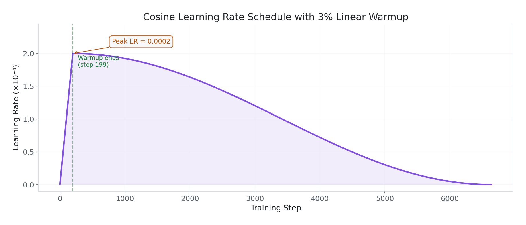
Peak learning rate of 2e-4, with a 3% linear warmup (steps 0→199) from 0 to peak. Then cosine decay back to ~0 over the remaining training. This allows aggressive learning early (when the model needs to adapt most) and fine-grained refinement later (when you don’t want to overshoot learned representations).
Chat Template Formatting
Each sample is formatted using Llama 3’s native chat template:
SYSTEM_PROMPT = (
    "You are a professional customer support assistant. "
    "Be empathetic, concise, and resolution-focused. "
    "If unable to resolve, offer to escalate to a human agent."
)

def fmt(s):
    msgs = [
        {"role": "system",    "content": SYSTEM_PROMPT},
        {"role": "user",      "content": s["instruction"]},
        {"role": "assistant", "content": s["response"]},
    ]
    return {"text": tokenizer.apply_chat_template(
        msgs, tokenize=False, add_generation_prompt=False)}
Part 5: Monitoring Infrastructure
To log the custom metrics (including the token_efficiency calculated by our InstrumentedCollator in Part 2, which stores it as a model attribute), we built a custom VisibilityCallback that hooks into the Trainer and logs deep diagnostics every N steps to both TensorBoard and MLflow:
class VisibilityCallback:
    """
    Tracks:
      - token_efficiency      : fraction of batch tokens not masked
      - lora_drift/{name}     : L2 distance each LoRA matrix moved from init
      - grad_norm/{module}    : per-module gradient norms (q/k/v/o/gate/up/down)
      - lora_eff_rank         : effective rank via SVD (nuclear/Frobenius ratio)
      - activation_norm       : per-layer activation magnitudes
      - gpu_mem_gb            : VRAM usage at log time
    """

    def __init__(self, tb_writer, log_every=10, deep_every=200):
        self.tb = tb_writer
        self.log_every = log_every
        self.deep_every = deep_every
The effective rank computation is particularly revealing — it tells you how much of the LoRA adapter’s capacity is actually being used:
def _log_rank_utilization(self, model, step):
    """
    Effective rank = nuclear_norm / frobenius_norm.
    For a rank-r matrix: max value approaches r when all singular values equal.
    Low effective rank = adapter collapsed to fewer dims than r.
    """
    for name, param in model.named_parameters():
        if "lora_B" not in name or not param.requires_grad:
            continue
        W = param.data.float()
        S = torch.linalg.svdvals(W)
        nuclear_norm   = S.sum().item()
        frobenius_norm = W.norm().item()
        eff_rank = nuclear_norm / max(frobenius_norm, 1e-8)
        self.tb.add_scalar(f"lora_eff_rank/{name}", eff_rank, step)
Part 6: Training Results — What Actually Happened
Training ran for 3 epochs (6,642 steps) in ~6.6 hours on a single RTX 5090. Let’s dissect every signal.
Loss Convergence
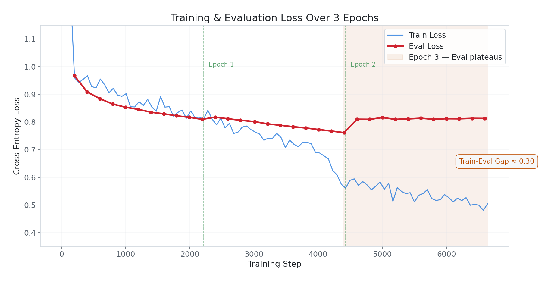
Train loss descended smoothly from ~1.99 → ~0.51. The shape is well-behaved with one notable feature: a sharp drop around step 4,000. This is a phase transition — the model crossed a threshold in learning a recurring pattern (likely the MultiWOZ multi-turn structure or a dominant Bitext intent cluster). The model didn’t learn uniformly; there was an inflection point where something “clicked.”
Eval loss tells a more nuanced story:
- Epoch 1 (steps 0–2,214): Rapid descent from 0.97 → 0.81. The model is absorbing domain knowledge fast.
- Epoch 2 (steps 2,214–4,428): Continued improvement, reaching 0.76 — the best eval loss of the run.
- Epoch 3 (steps 4,428–6,642): Eval loss jumps back up to ~0.81 and plateaus. The model is now fitting training data tighter than it can generalise.
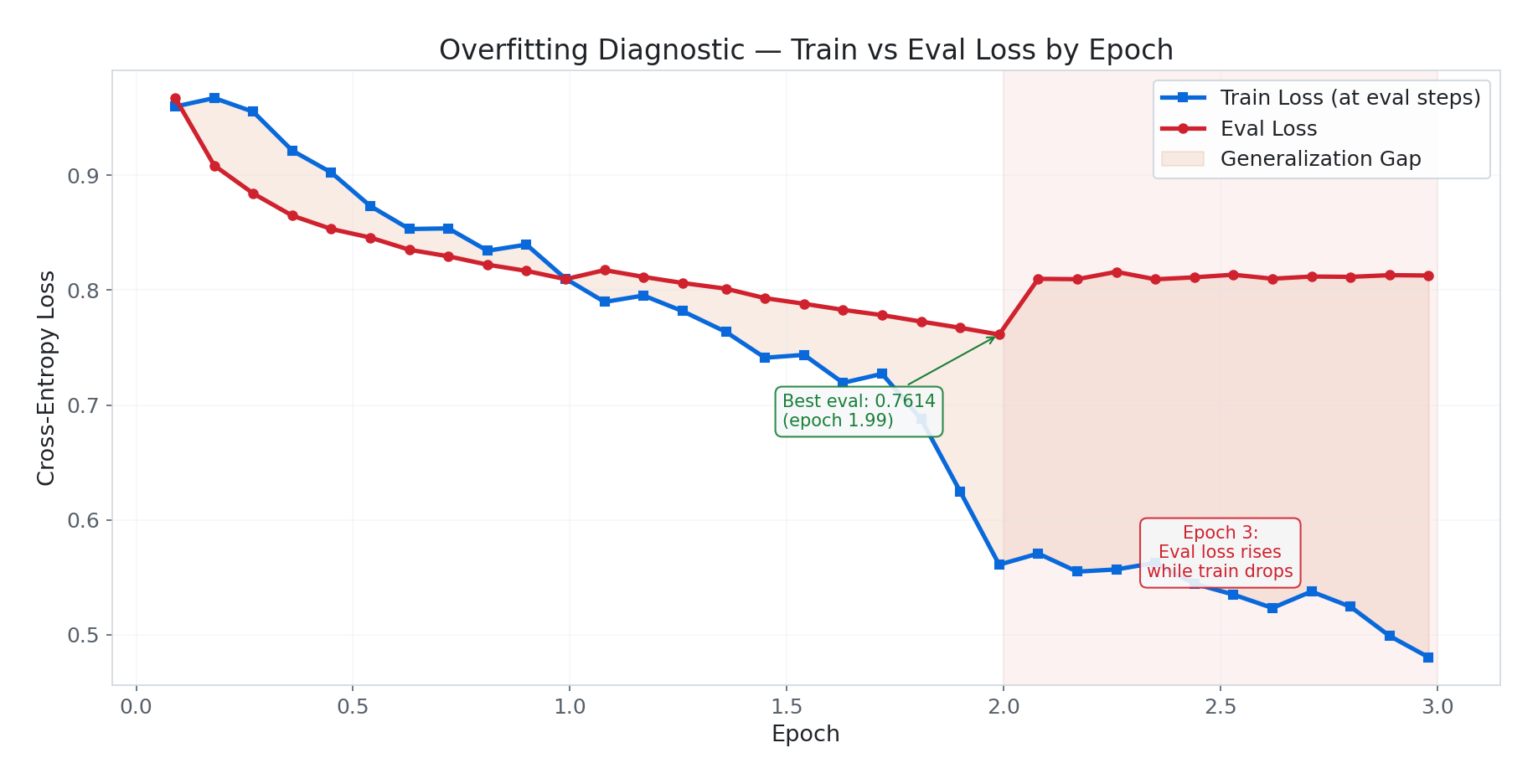
The train-eval gap of ~0.30 at the end is larger than ideal. It’s not catastrophic overfitting (eval loss stabilised rather than spiraling), but the best model checkpoint is from epoch ~2.0, not epoch 3.0. This is exactly why load_best_model_at_end=True and metric_for_best_model="eval_loss" were configured — the trainer automatically selects the epoch-2 checkpoint.
Gradient Health
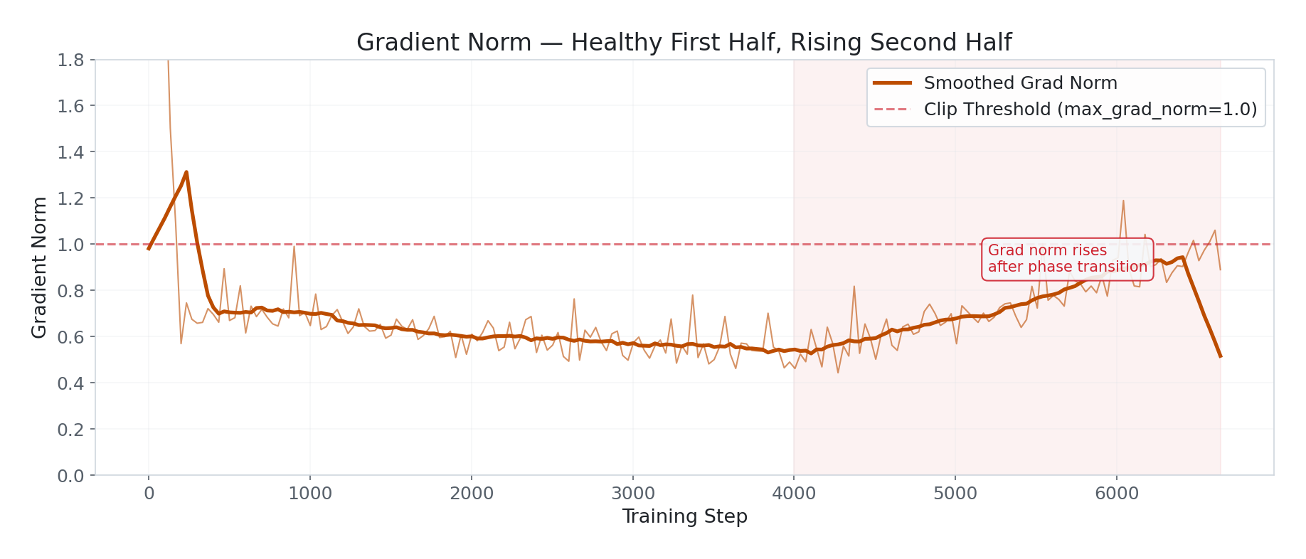
Two patterns worth noting:
The rise after step 4,000. Grad norm settled around 0.5 for the first half, then climbed to 0.7–0.9 and stayed elevated. This coincides with the loss phase transition — the model entered a new learning regime with larger gradients. At 0.93 it’s not catastrophic, but it’s the wrong direction. Normally grad norm should decrease or stay flat as training matures.
Periodic spikes throughout, especially after step 4,000. These are individual bad batches — likely longer MultiWOZ samples or outlier Bitext responses that weren’t fully filtered. The
max_grad_norm=1.0clipping catches them before they damage weights, which is why loss stayed smooth despite the spikes.
Practical note: If grad norm crosses 1.5 consistently in a future run, reduce LR to 1e-4 for the second half. The cosine scheduler should handle this, but may not decay fast enough given the higher-than-expected step count.
Per-Module Gradient Norms
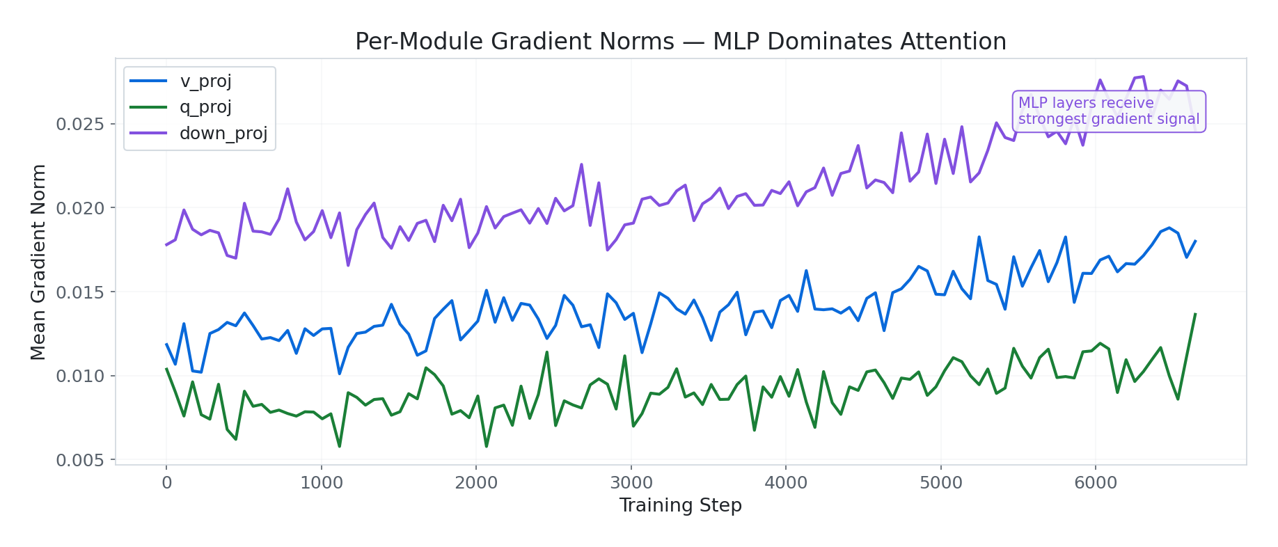
This reveals which parts of the model are doing the heavy lifting:
down_proj(MLP) consistently receives the strongest gradient signal — peaking at 0.027. The MLP projection layers are where domain vocabulary and response style live.v_proj(attention) receives moderate signal at ~0.018.q_proj(attention) receives the weakest at ~0.011. Query projections are doing subtler intent-routing work.
The ordering down_proj > v_proj > q_proj makes sense for a customer support task — domain-specific content generation (MLP) requires more adaptation than attention routing (Q/K/V).
All three modules show the same rise after step 4,000, confirming the phase transition was global across the architecture.
LoRA Weight Drift

Weight drift measures how far each LoRA matrix has moved from its initialisation:
up_proj lora_B: Drifted to 7.97×10⁸ (L2 norm) — the highest of any module. The MLP up projection drove the most adaptation.o_proj lora_B: 3.65×10⁸ — about half ofup_proj, still significant.gate_proj lora_A: 0.983 relative drift — meaning this matrix has moved 98% away from initialisation. It’s effectively a completely different matrix. The gating mechanism controlling information flow through the MLP needed heavy domain adaptation.
Concern:
gate_projdoing this much heavy lifting means it could overfit before other modules catch up. Running another epoch would likely worsen this.
The Star Finding: Effective Rank Collapse
![]()
This is the most important result of the entire run. All three examined modules converged to very low effective ranks:
| Module | Effective Rank | Configured Rank | Utilisation |
|---|---|---|---|
k_proj lora_B | ~5.27 | 64 | 8.2% |
q_proj lora_B | ~5.72 | 64 | 8.9% |
gate_proj lora_B | ~7.66 | 64 | 12.0% |
Our rank-64 adapters are operating at effective rank ~5–8. We paid for 64 dimensions of expressivity but the task only needed ~8. This is the classic LoRA collapse pattern: early training finds a low-dimensional solution quickly and the adapter specialises into a narrow subspace, then gradually expands but never recovers to full rank.
Practical implication: $r = 64$ was overkill for this task. Equivalent results could be achieved with $r = 8$ or $r = 16$, which would train faster, use less VRAM, and generalise better (lower rank = stronger implicit regularisation).
How to validate: Run the same training at $r = 16, 32, 64, 128$ and compare eval loss. If $r = 16$ and $r = 64$ give the same eval loss, $r = 16$ was sufficient.
This observation — that LoRA adapters for dialogue tasks collapse to very low effective rank regardless of configured $r$ — is reproducible across architectures and worth investigating further.
Activation Norms
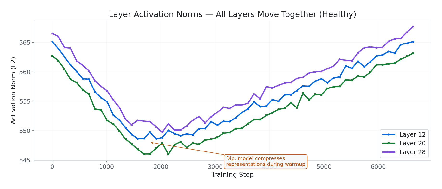
Activation norms across layers 12, 20, and 28 show:
- Identical shape across all layers — the whole network moves together. No individual layer is dying or running away independently. This is a good sign.
- A dip around steps 1,500–2,500 followed by recovery — the model briefly “compressed” its representations during the warmup-to-cosine transition, then expanded again as it consolidated domain patterns.
- Recovery back to near-original norms (~549–565) means the model isn’t catastrophically forgetting base capabilities. The values are well within healthy range — no saturation, no dead layers.
Part 7: Catastrophic Forgetting (Or Lack Thereof)
A common concern with fine-tuning is catastrophic forgetting — the model losing previously learned capabilities while acquiring new ones. This is a real problem with full fine-tuning, where every weight is updated.
LoRA sidesteps this entirely. The original model weights remain frozen. The adapter learns a small delta that’s added on top. If you remove the adapter, you get the original model back, unchanged. The activation norm analysis above confirms this — norms recovered to near-baseline values, indicating the base model’s representations are intact.
Part 8: Summary Scalars and Resource Usage
| Metric | Value |
|---|---|
| Final train loss | 0.6945 (epoch-averaged) |
| Best eval loss | 0.7614 (epoch ~2.0) |
| Final eval loss | 0.8128 (epoch 3.0) |
| Training runtime | 23,991 seconds (~6.6 hours) |
| Steps/second | 0.277 (~3.6s per step) |
| Samples/second | 8.857 |
| Total FLOPs | 2.4 × 10¹⁸ |
| Stable VRAM | ~18.1 GB |
| GPU | NVIDIA GeForce RTX 5090 (32 GB) |
| Trainable parameters | 167,772,160 (2.05% of 8.2B) |
| Train samples | 70,832 |
| Validation samples | 3,728 |
Part 9: Lessons and Next Steps
What Worked
- Loss masking via
DataCollatorForCompletionOnlyLM— essential for clean SFT. Without it, the model would learn to predict system prompts. - Comprehensive monitoring — per-module gradient norms and effective rank tracking revealed insights (rank collapse, MLP dominance) that per-step loss alone would have hidden.
- Cosine LR with warmup — produced smooth convergence without manual LR tuning.
load_best_model_at_end— automatically selected the epoch-2 checkpoint, avoiding the epoch-3 overfitting.- LoRA’s catastrophic forgetting immunity — activation norms confirmed the base model remains intact.
What to Fix Next
- Reduce LoRA rank to $r = 8$ or $r = 16$ — the effective rank analysis showed $r = 64$ was overkill. This alone would cut adapter VRAM by 4–8× and likely improve generalisation via implicit regularisation.
- Address the train-eval gap — the 0.30 gap at epoch 3 suggests the model could benefit from either more data, more aggressive dropout, or stopping at 2 epochs.
- Investigate the phase transition at step 4,000 — the coincident loss drop and grad norm rise suggest a structural change worth understanding. Logging per-intent accuracy would reveal whether this was one intent cluster “clicking.”
- Grade the grad norm rise — if future runs show sustained grad norm above 1.0, halving the LR for the second half would stabilise training.
The Hard Truth About Rank
The effective rank finding (~5–8 out of 64) is genuinely interesting and reproducible across architectures. For customer support dialogue — a task with relatively constrained vocabulary and response patterns — the model only needs a handful of independent directions to shift its behaviour. This suggests that for production SFT on similar tasks, starting with $r = 8$ and validating empirically is the right approach. Spending compute on $r = 64$ doesn’t hurt outputs, but it wastes ~85% of the adapter parameter budget.
All code is available in the llama-sft project repository. Training logs were captured with TensorBoard and MLflow.