 Before we had Large Language Models writing poetry, we had to teach computers that “king” and “queen” are related not just by spelling, but by meaning. This is the story of that breakthrough. It’s the moment we stopped counting words and started mapping their souls—turning raw text into a mathematical landscape where math can solve analogies. Welcome to the world of Word2Vec. 🔮
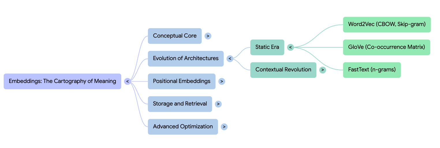
- Language models require vector representations of words to capture semantic relationships.
- Before the 2010s, models used word count-based vector representations that captured only the frequency of words (e.g., One-Hot Encoding).
The Problems: 🚧
- The Curse of Dimensionality
- Lack of meaning (Synonyms were treated as mathematically unrelated).
In 2011, Mikolov et al. at Google introduced Word2Vec, which used a shallow neural network to learn vector representations of words. The best part? It could create much denser relationships between words than prior models, and it was unsupervised.
The training (prediction) is essentially “fake”—a pretext task. But the weight matrices we get on the side are a gold mine of fine-grained semantic relationships. ⛏️
There are two popular variants of Word2Vec:
- SkipGram
- Continuous Bag Of Words (CBOW)
1. Continuous Bag of Words (CBOW) 🧩
CBOW is a simple ‘fill in the blanks’ machine. It takes the surrounding words as inputs and tries to predict the center word.
“Continuous”: It operates in continuous vector space (unlike the discrete space of n-gram models).
“Bag of words”: The order of the context does not matter. “The cat sat on the mat” and “The mat sat on the cat” are the same for CBOW. They produce exactly the same predictions.
Objective: Maximize the probability of the target word $w_t$ given its context $w_{t-C}, \dots, w_{t+C}$.
2. Training
Defining Dimensions:
- $V$: Vocabulary size (number of unique words in the corpus, e.g., 10,000)
- $N$: Dimension of the embedding space (e.g., 100)
- $C$: Number of context words (e.g., 2 words on left of target and 2 words on right)
Step 1: Input Lookup & One-Hot Encoding
Mathematically, we represent each context word as a one-hot vector $x^{(c)}$. We have an Input Matrix $W_{in}$ of size $V \times N$. For each context word (e.g., “The”, “cat”, “on”, “mat”), we select its corresponding row from $W_{in}$.
$$ v_c = W_{in}^T x^{(c)} $$
Where $v_c$ is the $N$-dimensional vector for context word $c$.
Step 2: Projection (The “Mixing”)
We combine the context vectors. In standard CBOW, we simply average them. This creates the hidden layer vector $h$.
$$ h = \frac{1}{2C} \sum_{c=1}^{2C} v_c $$
$h$ is a single vector of size $N \times 1$. Note: This operation is linear and contains no activation function (like ReLU or Sigmoid).
Step 3: Output Scoring (The “Dot Product”)
We have a second matrix, the Output Matrix $W_{out}$ of size $N \times V$. We compute the raw score (logit) $u_j$ for every word $j$ in the vocabulary by taking the dot product of the hidden vector $h$ and the output vector $v’_j$.
$$ u_j = {v’_j}^T h $$
Or in matrix form:
$$ u = W_{out}^T h $$
Result $u$ is a vector of size $V \times 1$.
Step 4: Probability Conversion (Softmax)
We convert the raw scores $u$ into probabilities using the Softmax function. This tells us the probability that word $w_j$ is the center word.
$$ y_j = P(w_j | \text{context}) = \frac{\exp(u_j)}{\sum_{k=1}^V \exp(u_k)} $$
Step 5: Loss Calculation (Cross-Entropy)
We compare the predicted distribution $y$ with the actual ground truth $t$ (a one-hot vector where the index of the true word is 1). The loss function $E$ is:
$$ E = - \sum_{j=1}^V t_j \log(y_j) $$
Since $t_j$ is 0 for all words except the target word (let’s call the target index $j^*$), this simplifies to:
$$ E = - \log(y_{j^*}) $$
3. Backpropagation Details
We need to update the weights to minimize $E$. We use the Chain Rule.
A. Gradient w.r.t. Output Matrix ($W_{out}$)
We want to know how the error changes with respect to the raw score $u_j$.
$$ \frac{\partial E}{\partial u_j} = y_j - t_j $$
Let’s call this error term $e_j$.
- If $j$ is the target word: $e_j = y_j - 1$ (Result is negative; we boost the score).
- If $j$ is not target: $e_j = y_j - 0$ (Result is positive; we suppress the score).
The update rule for the output vector $v’_j$ becomes:
($\eta$ is the learning rate)
B. Gradient w.r.t. Hidden Layer ($h$)
We backpropagate the error from the output layer to the hidden layer.
$$ EH = \sum_{j=1}^V e_j \cdot v’_j $$
$EH$ is an $N$-dimensional vector representing the aggregate error passed back to the projection layer.
C. Gradient w.r.t. Input Matrix ($W_{in}$)
Since $h$ was just an average of the input vectors, the error $EH$ is distributed to each context word’s input vector. For every word $w_c$ in the context:
$$ v_{w_c}(\text{new}) = v_{w_c}(\text{old}) - \eta \cdot \frac{1}{2C} \cdot EH $$
Let’s build a single pass through the network for a given context.
import torch
import torch.nn as nn
import torch.nn.functional as F
import torch.optim as optim

# Define a simple Continuous Bag of Words (CBOW) style model
class CBOWModel(nn.Module):
    def __init__(self, vocab_size, embedding_dim):
        super(CBOWModel, self).__init__()
        # The embedding layer stores the word vectors we want to learn
        self.embeddings = nn.Embedding(vocab_size, embedding_dim)
        # The linear layer maps the averaged embedding back to the vocabulary size to predict the target word
        self.linear = nn.Linear(embedding_dim, vocab_size)

    def forward(self, inputs):
        # inputs: tensor of word indices for the context
        embeds = self.embeddings(inputs)
        # Aggregate context by calculating the mean of the word embeddings
        h = torch.mean(embeds, dim=1)
        # Produce logits (raw scores) for each word in the vocabulary
        logits = self.linear(h)
        return logits

# Setup vocabulary and mappings
word_to_ix = {"the": 0, "quick": 1, "brown": 2, "fox": 3, "jumps": 4, "over": 5, "lazy": 6, "dog": 7}
ix_to_word = {v: k for k, v in word_to_ix.items()}

# Configuration constants
EMBEDDING_DIM = 5
VOCAB_SIZE = len(word_to_ix)
LEARNING_RATE = 0.01

# Initialize the model, loss function, and optimizer
model = CBOWModel(VOCAB_SIZE, EMBEDDING_DIM)
loss_function = nn.CrossEntropyLoss()
optimizer = optim.SGD(model.parameters(), lr=LEARNING_RATE)

# Prepare dummy training data: context words and the target word
# Context: ["quick", "brown", "jumps", "over"] -> Target: "fox"
context_idxs = torch.tensor([1, 2, 4, 5], dtype=torch.long)
target_idxs = torch.tensor([3], dtype=torch.long)

# Perform a single optimization step
model.zero_grad()
# Forward pass: we reshape context to (1, -1) to simulate a batch of size 1
logits = model(context_idxs.view(1, -1))
# Calculate loss against the target word index
loss = loss_function(logits, target_idxs)
# Backpropagate and update weights
loss.backward()
optimizer.step()

# Output results for the blog post
print("=== Model Training Snapshot ===")
print(f"Calculated Loss: {loss.item():.6f}")

print(f"\n=== Learned Vector for 'jumps' ===")
word_vec = model.embeddings(torch.tensor([word_to_ix['jumps']]))
print(word_vec.detach().numpy())

print("\n=== Embedding Matrix (Weights) ===")
print(model.embeddings.weight.detach().numpy())

print("\n=== Linear Layer Weights ===")
print(model.linear.weight.detach().numpy())
Output shows single pass loss and learned vector for ‘jumps’ word. This is a single training sample result but after multiple such passes both Embedding and linear weights should be very similar.
=== Model Training Snapshot ===
Calculated Loss: 1.989656

=== Learned Vector for 'jumps' ===
[[-1.5040519  -0.5602162  -0.11328011 -0.67929274 -0.84375775]]

=== Embedding Matrix (Weights) ===
[[ 1.66039    -0.11371879  0.6246518   0.35860053 -1.2504417 ]
 [-2.1847186  -0.77199775 -0.17050214 -0.38411248 -0.03913084]
 [ 0.11852697  0.90073633  0.8847807   0.7404524   0.900149  ]
 [ 0.07440972 -0.40259898  2.6246994  -0.08851447  0.02660969]
 [-1.5040519  -0.5602162  -0.11328011 -0.67929274 -0.84375775]
 [-0.9245572  -0.5545908   0.9083091  -1.0755049   0.84047747]
 [-1.0237687   0.59466314  0.05621134 -0.6202532   1.3664424 ]
 [ 0.60998917 -1.0549186   1.6103884   0.8724912  -1.2486908 ]]

=== Linear Layer Weights ===
[[ 0.02165058 -0.28883642  0.14545658 -0.3442509   0.32704315]
 [-0.18731792  0.28583744  0.22635977  0.13245736  0.29019794]
 [ 0.3158916  -0.15826383 -0.03203773  0.16377363 -0.41457543]
 [-0.05080034  0.4180087   0.11228557  0.30218413  0.3025514 ]
 [-0.38419306  0.24475925 -0.39210224 -0.38660625 -0.2673145 ]
 [-0.32321444  0.12200444 -0.03569533  0.2891424  -0.07345333]
 [-0.33704326  0.2521956   0.31587374  0.22590035  0.29866052]
 [ 0.4117266  -0.44231793  0.24064957 -0.29684234  0.333821  ]]
Interesting Facts About CBOW 🧠
The “Averaging Problem”: This is a common issue in CBOW models. The averaging and training is order-agnostic. All variants of word order in the context window will generate the same output. “Dog bit the man” and “Man bit the dog” are the same in CBOW’s eyes.
Smoothing Effect: CBOW models are much faster to train than Skip-Gram but are generally smoother.
Rare Words: CBOW models struggle slightly with rare words because the presence of surrounding common words (like articles and prepositions) can skew the embeddings and dissolve their uniqueness.
Computational Cost: Softmax requires summing over the entire vocabulary size, which can be computationally expensive if $V$ is very large. Solutions include Hierarchical Softmax and Negative Sampling (approximating the denominator by only checking the target word vs. 5 random noise words).
Vectors as Double Agents: Every word has a different representation in the embedding matrix and the output matrix. Most of the time $W_{out}$ is discarded, but some consider averaging both $W_{in}$ and $W_{out}$ for slightly better performance.
Linear Relationships: The famous analogy
King - Man + Woman = Queenemerges from the model because of the linear relationships between the words.Initialization: This is a no-brainer but worth mentioning. Initialization to zero vectors would mean no learning. We must initialize randomly.
2. Skip-Gram (The “Burger Flip” of CBOW) 🔄
Skip-Gram flips the CBOW logic. While CBOW tries to predict the center word given the context, Skip-Gram tries to predict the scattered context given the center word.
Core Concept: If a word like “monarch” can accurately predict words like “king”, “throne”, “crown”, “royalty”, and “power”, then it must effectively capture the concept of royalty.
Training
Let’s define dimensions:
- $V$: Vocabulary size
- $D$: Embedding dimension
- $C$: Number of context words
Step 1: Input Lookup
Unlike CBOW, our input is just one word vector (the center word $w_t$). We grab the vector $v_c$ from the Input Matrix $W_{in}$.
$$ h = v_{w_t} $$
Note: There is no averaging here. The hidden layer $h$ is simply the raw vector of the center word.
Step 2: Output Scoring (The Broadcast)
The model takes this single vector $h$ and compares it against the Output Matrix $W_{out}$ (the entire vocabulary). It computes a score $u_j$ for every word $j$ in the dictionary.
$$ u = W_{out}^T h $$
Result $u$: A vector of size $V \times 1$ containing raw scores.
Step 3: Probability Conversion (Softmax)
We apply Softmax to turn scores into probabilities.
$$ P(w_j | w_t) = \frac{\exp(u_j)}{\sum_{k=1}^V \exp(u_k)} $$
Step 4: The Multi-Target Loss
Here is the major difference from CBOW. In CBOW, we had one target (the center). In Skip-Gram, we have $2C$ targets (all the surrounding words). For a sentence “The cat sat on mat” (Center: “sat”), the targets are “The”, “cat”, “on”, “mat”. We want to maximize the probability of all these true context words. The Loss function ($E$) sums the error for each context word:
$$ E = - \sum_{w_{ctx} \in \text{Window}} \log P(w_{ctx} | w_t) $$
Step 5: Backpropagation (Accumulating Gradients)
Since one input word is responsible for predicting multiple output words, the error signals from all those context words add up.
At the Output Layer:
- If “cat” was a target, the “cat” vector in $W_{out}$ gets a signal: “Move closer to ‘sat’.”
- If “apple” was NOT a target, the “apple” vector gets a signal: “Move away from ‘sat’.”
At the Hidden Layer ($h$):
- The center word “sat” receives feedback from all its neighbors simultaneously.
- Error signal = (Error from “The”) + (Error from “cat”) + (Error from “on”)…
- The vector for “sat” in $W_{in}$ moves in the average direction of all its neighbors.
3. The “Computational Nightmare” & Negative Sampling
The equations above describe Naive Softmax.
The Problem: If $V = 100,000$, computing the denominator $\sum \exp(u_k)$ takes 100,000 operations. Doing this for every word in a training set of billions of words is impossibly slow.
The Solution: Negative Sampling Instead of updating the entire vocabulary (1 correct word vs 99,999 wrong ones), we approximate the problem.
- Positive Pair: (sat, cat) $\rightarrow$ Maximize probability (Label 1).
- Negative Pairs: We pick $K$ (e.g., 5) random words the model didn’t see, e.g., (sat, bulldozer), (sat, quantum). $\rightarrow$ Minimize probability (Label 0).
New Equation (Sigmoid instead of Softmax):
Effect: We typically only update 6 vectors per step (1 pos + 5 negs) instead of 100,000.
Let’s see this in code:
import torch
import torch.nn as nn
import torch.optim as optim

class SkipGramNegativeSampling(nn.Module):
    """
    Skip-Gram with Negative Sampling (SGNS) implementation.

    SGNS approximates the softmax over the entire vocabulary by instead
    distinguishing between a real context word (positive) and K noise words (negative).
    """
    def __init__(self, vocab_size, embedding_dim):
        super(SkipGramNegativeSampling, self).__init__()
        # Input embeddings: used when the word is the center word
        self.in_embed = nn.Embedding(vocab_size, embedding_dim)
        # Output embeddings: used when the word is a context or negative sample
        self.out_embed = nn.Embedding(vocab_size, embedding_dim)

        # Initialize weights with small values to prevent gradient saturation
        initrange = 0.5 / embedding_dim
        self.in_embed.weight.data.uniform_(-initrange, initrange)
        self.out_embed.weight.data.uniform_(-initrange, initrange)

    def forward(self, center_words, target_words, negative_words):
        """
        Computes the negative sampling loss.

        Args:
            center_words: (batch_size)
            target_words: (batch_size)
            negative_words: (batch_size, K) where K is number of negative samples
        """
        # Retrieve vectors
        v_c = self.in_embed(center_words)      # (batch_size, embed_dim)
        u_o = self.out_embed(target_words)     # (batch_size, embed_dim)
        u_n = self.out_embed(negative_words)   # (batch_size, K, embed_dim)

        # 1. Positive Score: log(sigmoid(v_c · u_o))
        # Compute dot product: (batch, 1, dim) @ (batch, dim, 1) -> (batch, 1)
        pos_score = torch.bmm(u_o.unsqueeze(1), v_c.unsqueeze(2)).squeeze(2)
        pos_loss = torch.log(torch.sigmoid(pos_score) + 1e-7)

        # 2. Negative Score: sum(log(sigmoid(-v_c · u_n)))
        # Compute dot products for all K samples: (batch, K, dim) @ (batch, dim, 1) -> (batch, K)
        neg_score = torch.bmm(u_n, v_c.unsqueeze(2)).squeeze(2)
        neg_loss = torch.sum(torch.log(torch.sigmoid(-neg_score) + 1e-7), dim=1, keepdim=True)

        # Total loss is the negative of the objective function
        loss = -(pos_loss + neg_loss)
        return torch.mean(loss)

# --- Configuration & Mock Data ---
VOCAB_SIZE = 100
EMBED_DIM = 10
word_to_ix = {'fox': 0} # Example vocabulary mapping

model = SkipGramNegativeSampling(VOCAB_SIZE, EMBED_DIM)
optimizer = optim.SGD(model.parameters(), lr=0.01)

# Mock inputs: 1 center word, 1 target word, 5 negative samples
center_id = torch.tensor([0], dtype=torch.long)
target_id = torch.tensor([1], dtype=torch.long)
negative_ids = torch.tensor([[50, 23, 99, 4, 12]], dtype=torch.long)

# Training Step
model.zero_grad()
loss = model(center_id, target_id, negative_ids)
loss.backward()
optimizer.step()

# Output Results
print(f"Loss after one step: {loss.item():.6f}")
word_vec = model.in_embed(torch.tensor([word_to_ix['fox']]))
print(f"Vector for 'fox':\n{word_vec.detach().numpy()}")
The outputs:
Loss after one step: 4.158468
Vector for 'fox':
[[ 0.04197385  0.02400733 -0.03800093  0.01672485 -0.03872231 -0.0061478
   0.0121122   0.04057864 -0.036255    0.03861175]]
Interesting Facts About Skip-Gram 💡
Makes Rare Words Shine: Skip-Gram is more effective at capturing the meaning of rare words because it focuses on the context of the center word. In CBOW, a rare word’s vector is averaged with others, diluting its signal. In Skip-Gram, when the rare word appears as the center, it gets the full, undivided attention of the backpropagation update.
Slow Training: This method creates more training samples. A window of size 2 creates 4 training pairs per center word, while CBOW creates only 1 training pair per center word.
Semantic Focus: Skip-Gram puts more emphasis on the semantic relationship between words. It views the context as the primary signal, with the center word as the target. This makes it better at capturing the meaning of words in context. Skip-Gram tends to capture semantic relationships (King/Queen) slightly better, while CBOW captures syntactic ones (walk/walked) slightly better.